Adaptive Step Sizes and TCP Retransmission Timers

Code for the figure lives in the companion repo: johnnyli-dev/blog-simulations.

This past semester I took Math 128A (Numerical Analysis) and CS 168 (Introduction to the Internet: Architecture and Protocols). Towards the end of the semester while I was studying for finals it saw how the RK45 adaptive step controller and the Jacobson/Karels RTO estimator looked and felt almost the same. Both algorithms watch a noisy quantity, keep a running estimate of how noisy it is, and set a single control parameter as "best guess plus a margin scaled by some unsureness factor." The two algorithms live in completely different settings, so what is interesting is not that they look similar but where my attempt at making an analogy fails.

Adaptive step sizes in RK45

A fixed-step Runge-Kutta method has no way to know whether the current step is wasting effort on a smooth region or missing a sharp transition. The Fehlberg/Dormand-Prince trick is to compute two approximations at every step using the same intermediate slope evaluations: one of order 5 and one of order 4. Compute is cheap because they share computations and thus only require a select few more calculation to go from order 4 to 5. We then take the difference between the estimates and the local truncation error of the lower-order method, call this $\mathrm{err}$. This is our embedded estimator. It is essentially free, and it gives a real measurement of how wrong the step was, not a bound.

Given a user tolerance $\mathrm{tol}$, the controller picks the next step size by demanding that the predicted error stay near $\mathrm{tol}$. Since the local error of a method of order $p$ scales like $h^{p+1}$, the update rule is

with $p = 4$ for the lower-order method, so the exponent is $1/5$. The safety factor of $0.9$ keeps the controller from skating right up to the tolerance and tripping. If $\mathrm{err} > \mathrm{tol}$, the step is rejected, $h$ is shrunk by the same formula, and the step is retried from the previous point. If $\mathrm{err}$ is comfortably below $\mathrm{tol}$, the same formula tells the solver to take a bigger step next time.

The thing to hold onto is that RK45 gets a clean, deterministic measurement of its own error at every step. The controller does not have to guess. It can be aggressive in both directions because the feedback is sharp.

Jacobson/Karels RTO

On the networking side we have TCP, and it has the opposite problem. The sender needs a retransmission timeout: long enough that real round trips do not falsely fire, short enough that a genuinely lost packet does not stall the connection. Before Jacobson, the standard was a low-pass filtered round-trip estimate $\mathrm{SRTT}$ and a fixed multiplier, $\mathrm{RTO} = \beta \cdot \mathrm{SRTT}$ with $\beta \approx 2$. This works fine on a quiet link. Under congestion, RTTs do not just rise, they fan out, and a fixed multiplier on the mean is far too tight against the new variance. The result is spurious retransmissions, which pile more traffic onto an already congested link, which raises RTTs further. The 1986 NSFnet collapse traced back to exactly this loop.

Jacobson and Karels fixed it by tracking variability explicitly. On each RTT sample $R$:

with $\alpha = 1/8$ and $\beta = 1/4$. $\mathrm{SRTT}$ is an exponentially weighted mean of past RTTs, $\mathrm{RTTVAR}$ is an exponentially weighted mean absolute deviation, and the timeout is the mean plus four deviations. When the path is calm, $\mathrm{RTTVAR}$ decays and $\mathrm{RTO}$ hugs $\mathrm{SRTT}$. When queueing bursts hit, $\mathrm{RTTVAR}$ jumps and $\mathrm{RTO}$ widens to absorb the new spread before the controller has even decided what the new mean is.

Two more pieces matter. The first is Karn's algorithm: do not sample RTT from a retransmitted segment, because you cannot tell whether the ACK is for the original or the retransmission, and using either guess will systematically bias the estimator. The second is exponential backoff: when an RTO actually fires, double it before retrying. Both rules exist because TCP cannot run an embedded estimator. Sending a probe packet to measure how loaded the network is would itself load the network. So TCP has to estimate from the same sparse, ambiguous samples that carry its real traffic, and it has to fall back to crude heuristics in exactly the regimes where samples are most corrupted.

The structural parallel

Both algorithms maintain three things: a running estimate of an unobservable quantity (the true local error, the true RTT distribution), a running estimate of its variability ($\mathrm{err}$ itself for RK45, $\mathrm{RTTVAR}$ for TCP), and a single control parameter set at "current estimate plus a margin scaled by the variability." Both expand the control parameter aggressively when the underlying process gets harder and contract it when it gets easier. The figure below shows the same shape from two angles.

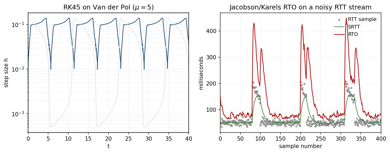
The left panel solves the Van der Pol oscillator at $\mu = 5$, which has stiff transition regions where the solution swings fast and long quiet stretches where it barely moves. The RK45 step size drops by two orders of magnitude through each transition and climbs back up through each smooth stretch. The right panel runs Jacobson/Karels on a lognormal RTT stream with three injected queueing bursts. $\mathrm{RTO}$ tracks $\mathrm{SRTT}$ closely when the path is quiet, then jumps with $\mathrm{RTTVAR}$ during each burst and decays as the variability estimate forgets the spike. Both controllers react asymmetrically: they widen fast when wrong and narrow slowly when calm, because the cost of an under-estimate (a missed transient, a spurious retransmit) is worse than the cost of an over-estimate (a few wasted steps, a slightly slow recovery).

Where the analogy breaks

The two settings are not symmetric, and the asymmetry is the whole reason TCP looks the way it does. RK45 has a deterministic ODE with known smoothness structure, and the embedded estimator gives it a real per-step error signal almost for free. TCP has a stochastic, non-stationary process and no free error signal. Its only feedback that the timer was wrong is a timeout, which is exactly the event whose probability the timer is trying to control. The parts of TCP that feel ad hoc to a numerical analyst are the parts that exist because the clean feedback loop is not available. The multiplier of $4$ on $\mathrm{RTTVAR}$ is not derived from a Gaussian quantile, it is just a number that worked. Karn's rule is there because the sampling process is ambiguous. Exponential backoff is there because once the timer has actually fired, the estimator has lost its grip and a multiplicative retreat is the cheapest safe move. Reading the two algorithms next to each other, the lesson I took was not that they are the same algorithm in different clothes but that the deterministic version is much smaller. Most of the apparent complexity in TCP is paying for the fact that the network will not tell it the truth.

Close

What the comparison gave me was a cleaner way to read each algorithm. RK45 is the simple case of a control problem TCP solves under adversarial conditions, and the heuristics in TCP are not arbitrary, they are the specific places where the simple case stops applying.